Introduction

In the world of machine learning research the top dogs have all the fun. They designed the preeminant architecture to scale to as many GPUs as possible. They command small armies of servers that scrape massive datasets. They are fiercly protective. Unfortunately it seems that AGI will be behind an API.

But there is a glimmer of hope for the GPU poor. Non generative models are smaller and more efficient to train. I train a ViT-S from scratch using a super efficient technique. I did all experiments using one underclocked RTX-3090. I discuss my design choices and their implications.

Motivation

Pretraining an image encoder from scratch is expensive. The reigning techniques requires somewhere in the ballpark of 300 A100 GPU-hours. An A100 GPU-hour is a unit which means using one A100 GPU for one hour. If you have 300 A100 GPUs it will take you one hour to spend 300 A100 GPU-hours. Each A100 GPU-hour costs about $1 on vastai. So the cost of training an image encoder from scratch is about $300. But this figure only includes one single training run. It does not include GPU-hours wasted on debugging code and tuning hyperparameters [note] The training run itself can be a small percentage of total compute if you are researching a new technique and you need to test different settings. For example, the DINOv2 paper estimated that they used just shy of 5 million A100 GPU hours in total compared to the 22 thousand for their largest ViT-G. .

Is this high cost an intrinsic quality of training image encoders? Or is it a property of the research that is published? Researchers maximize benchmark results achievable under their compute constraints. If your lab commands an expensive cluster of GPUs, you will probably be researching techniques that best utilize the cluster. The most ubiquitous techniques came from well funded labs. This is bad for the GPU poor because this leaves the lower end of the pareto front unexplored.

I suspect that it does not actually require 300 GPU hours to train a good image encoder. The prevailing techniques are not optimized for low resource settings. It is important to have efficient techniques. Better low-scale efficiency could unlock different personalization techniques. There is demand for small custom models trained on custom data. This report is a first attempt to make some sense of the low resource landscape.

Architecture and Pretraining Objective

Archtecture

I use a ViT trained on mixed resolution images.

Why not a CNN? CNNs can be applied to varying resolution images one by one. But can't process them in batches. In order to reach high throughputs images have to be processed in uniformly sized batches. Transformer based vision networks can process images of varying resolutions in uniform batches. NaViT showed that training transformer models in this way is an effective strategy.

NaViT works by packing different images into uniform length sequences. You have to mask the attention matrix to ensure that tokens from a given image can only attend to tokens from the same image. You are able to adjust a knob which controls the balance between image size and image throughput. If you want to process more images, you can lower the overall resolution. Conversely raising the image resolution restricts you to lower training throughputs.

NaViT's controllable dial of throughput vs quality is an extremely powerful lever. If I twist the dial to maximize throughput, my 3090 GPU can do the forward backward and update step of a ViT-S at 2,000 images per second. Increasing the resolution drastically lowers the throughput but lets the model see the finer details.

Pretraining Objective

With NaViT as my architecture, I am free to choose a pretraining objective. Different pretraining objectives have different trade-offs in compute and quality. The best is the one that gets the highest benchmark results after being training for however many GPU-hours you have in your budget. There were a few options that I considered as potential pretraining objectives.

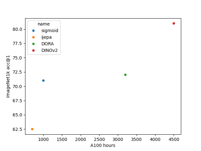
• Sigmoid Loss for Language Image Pre-Training: This is a contrastive method which learns a joint embedding space for images and texts. They get 71% zero shot accuracy on imagenet 1k after training with about 1,000 A100-hours [note] This assumes that 1 TPUv4 is roughly equivalent to 1 A100
• Self-Supervised Learning from Images with a Joint-Embedding Predictive Architecture This is a method that uses masked latent prediction. They report 62.5% accuracy on imagenet 1k using a linear probe. This is after training with about 700 A100-hours [note] Figure 5, ViT-B/16 .
• Is ImageNet worth 1 video? Learning strong image encoders from 1 long unlabelled video This is a method trained on a small number of long videos. They get 72% on imagenet 1k after training with 3,200 A100-hours [note] The authors state in their openreview comment that the (DORA ViT-S), when using 8 A100 GPUs, takes 6 hours and 48 minutes to train one epoch of ImageNet1k. Table 10 shows a model trained for 60 epochs obtaining 71.9% accuracy using a linear probe. .
• DINOv2: Learning Robust Visual Features without Supervision get 81% accuracy on imagenet after using 4,500 A100-hours. [note] The authors report that the ViT-S required 4,500 A100 hours to train. It also was not trained from scratch because it requires a larger pretrained model for distillation loss. I can't find where they report the training time for the ViT-S without distillation.

My budget was 100 A100 hours. For that budget I figured my best bet was to use IJEPA. IJEPA is new and untested. There are only four prominent research papers that trained image models using the technique described in IJEPA. [note] As of June 2024, to my best knowledge:

• Self-Supervised Learning from Images with a Joint-Embedding Predictive Architecture
• Learning and Leveraging World Models in Visual Representation Learning
• Stochastic positional embeddings improve masked image modeling
• DMT-JEPA: Discriminative Masked Targets for Joint-Embedding Predictive Architecture rejected from ICLR 2024

How does IJEPA work? Basically, the goal is to train a machine learning model that can understand images. You initialize with a random model. You give it an image with some missing rectangles. Seperately and secretly, you also give it the whole image. It's scored on how well it can predict it's own internal thoughts had it been able to see the entire image.

Implementation

I release the code and weights on github with an open license here: IJEPA-enhanced

Specs:
• GPU: 3090 with stock cooler, power limited to 250 watts
• CPU: AMD Ryzen 3700xt 8 cores
• RAM: 24 GB of DDR4 3200 MHz
• Storage: Cheap 1TB NVME SSD

Resolution sampling

IJEPA-enhanced uses random resolution sampling. I select the side resolution of an image by sampling from a uniform distribution. I use the sampled side resolution to obtain a height and width that maintains the aspect ratio of the original image. The resized height and resized width must be less than or equal to the original height and width. I crop the image at a random position using this height and width. Cropping is not the only way to obtain an image of a desired height and width. I also tried bilinear aspect-ratio-preserving resizing, which I found to be inferior [note] . For evaluation, I do not crop but instead resize the image, again maintaining aspect ratio. I do not use any additional image augmentations.

For my base experiment I set the min and max of the uniform distribution to be (70, 224). I then use a resolution of 252 for evaluation. Even though the evaluation resolution is higher than the training resolution, the model is able to extrapolate to higher resolutions and the higher resolution results in better imagenet1k linear probe accuracy.

Another important detail, as an offline preprocessing step, I resize all Imagenet1K training and validation images so that the largest side resolution is at most 256. This unlocks higher training throughputs because it lowers the cost of reading the images from the SSD.

Masking and packing

The masking strategy used by IJEPA plays to the strengths of sequence packing. Uniform sequence dimensions allows torch.compile and gives a big speedup. Furthermore, it allows for unique masks for each image.

I generate masks in the data loading pipeline. Each image has its own individual prediction masks. I sample 3 rectangles with scale uniformly distributed from 0.15 to 0.2 and aspect ratio from 0.75 to 1.5. I then randomly sample their positions. The tokens masked by the 3 rectangles are the prediction targets. I ensure that the union of the 3 masks has at least 1 patch and that the union of the 3 masks does not cover the entire image. Otherwise I start over and sample the masks again.

Then I greedily pack the tokens into batches. To pack a given sequence, I look at the length of the prediction tokens, and the length of the context tokens [note] Prediction tokens are tokens that are masked by any of the 3 target masks. The context tokens are all other tokens . The sequence is placed in the first available position in the batch where the prediction length is less than the max prediction length, and the context length is less than the max context length. If the sequence does not fit into any position in the batch, the prediction tokens are padded to the max prediction length and the context tokens are padded to the max context length, yielding a batch of shape (batch size, context length + prediction length, -1). This batch has context tokens (or padding) in batch[:, 0:context length, :] and has prediction tokens (or padding) in batch[:, context length:, :].

All packing is done by background workers. I use a smaller packer batch size and then combine the result of multiple packers to form a single full batch. Using this strategy, 9% of all of the context and target tokens are padding. I pack tokens into the context batch with a sequence length of 192, and target tokens into the target batch with a sequence length of 128.

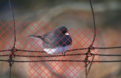
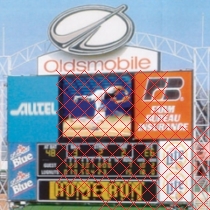
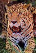
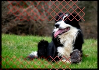
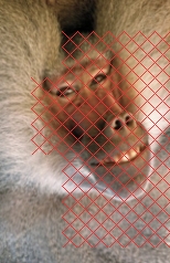
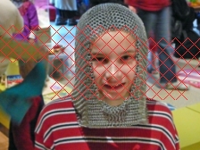
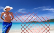
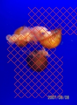
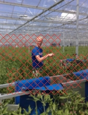
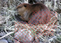
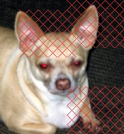
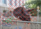
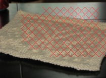
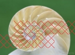
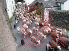
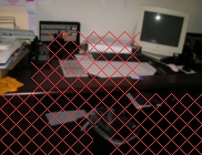
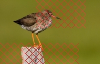
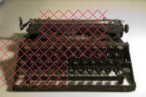
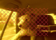
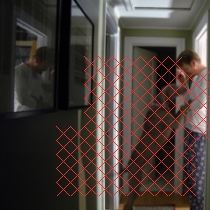
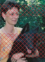
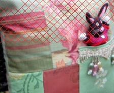
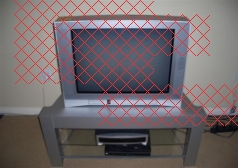
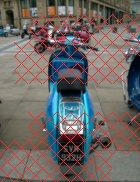
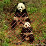
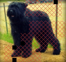
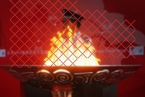
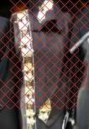
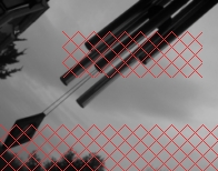
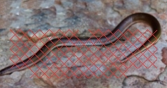
Training Image Samples

Here are several random training images. The pink zigzag lines indicate the masked tokens. Each "X" is one token. The student encoder gets to see all non masked tokens. The teacher encoder gets to see all original tokens. The predictor recieves the embeddings from the student encoder and also gets to see the positions of the masked tokens. The black tokens regions are dropped tokens. Some tokens were randomly dropped to fit the context or prediction tokens into the maximum sequence length.

Token Merging

Token merging (TOME) is a technique that aims to reduce the sequence length of the intermediate tensors that are processed by ViTs. It has been used as a post training method to speed up inference. But it also works to apply it during training. TOME merges or drops tokens that are similar, keeping the most distinct tokens. For IJEPA-enhanced, token merging addresses two points. 1.) Reducing the sequence length throughout model layers. 2.) Getting rid of superfluous noisy tokens when computing IJEPA loss.

The vanilla IJEPA loss is applied per token, similar to iBOT. Very eary research that shows that the teacher embeddings of iBOT has spatial inconsistencies [note] Morphing Tokens Draw Strong Masked Image Models https://arxiv.org/html/2401.00254v2 . The vanilla JEPA loss is probably too devoted to measuring WHERE information is, and not as devoted to measuring WHAT information there is [note] Demonstrated by Stochastic positional embeddings improve masked image modeling . Token merging prevents the model from embeddings that are spatially noisy. [note] Another work has tried to address the same issue with spatial noise using dynamic computation of targets, DMT-JEPA: Discriminative Masked Targets for Joint-Embedding Predictive Architecture, https://arxiv.org/abs/2405.17995

I use the technique described by Token Merging: Your ViT But Faster but I use token dropping instead of token merging. I use TOME not only to increase training throughput, but to beat the semantic objective vanilla IJEPA. I hypothesized that TOME would increase linear probing accuracy, even when controlling for throughput. In my experiments I found that there was a very small drop in linear probing accuracy when training with TOME, controlling for throughput.

I test two variations of TOME when computing IJEPA loss. The first variation is to unmerge tokens at the output of the teacher and student. This means that despite having internal hidden states with smaller sequence lengths, the outputs tokens have the same sequence length as the input tokens. I call this configuration `w unmerge`.

The second variation is to not unmerge at the output layer. The teacher takes as input `s` tokens, and returns about `s/2` tokens (depending on the `tome_r` parameter). The student also returns a lower number of tokens than it was inputted. This makes it difficult to deal with the predictor's position embeddings. Each input token to the predictor can be formed by one or more tokens of the original image. What are the (height,width) positions of these tokens? They are certainly not whole integers, so it does not make sense to use a embedding table. I deal with this by merging the position embeddings of the encoder. When the predictor is given an token, the position embeddings it recieves for that token are an average of the encoder's position embeddings of all of the input tokens it is composed of. Additionally there is a question of how to deal with the prediction mask. The prediction tokens are the ones not given to the context encoder; they are defined by a mask that masks the original unmerged tokens. Which merged tokens should be predicted? I choose to merge the prediction mask and set any merged token that is formed by at least one prediction token to be a prediction token. In practice this increases the percent of tokens from the teacher output that are masked. I call this configuration `wo unmerge`.

Using TOME, the teacher gets to leak a small amount of extra information to the predictor about the relationship between tokens. In vanilla IJEPA the predictor only gets to observe two things about masked tokens. Whether they exist in the first place, and what their positions are. In `wo unmerge` the position of the masked tokens are an almalgamation of the tokens that it was merged from. If masked tokens are part of a slobbering dog head, you'd expect some of the tokens that were merged to be roughly in the shape of the dog and his head. The way that the tokens are merged can indicate basic shapes and outlines that exist in the unmasked image. This contrasts to `w unmerge` where the predictor cannot as easily infer which tokens were merged in the teacher.

Diagram

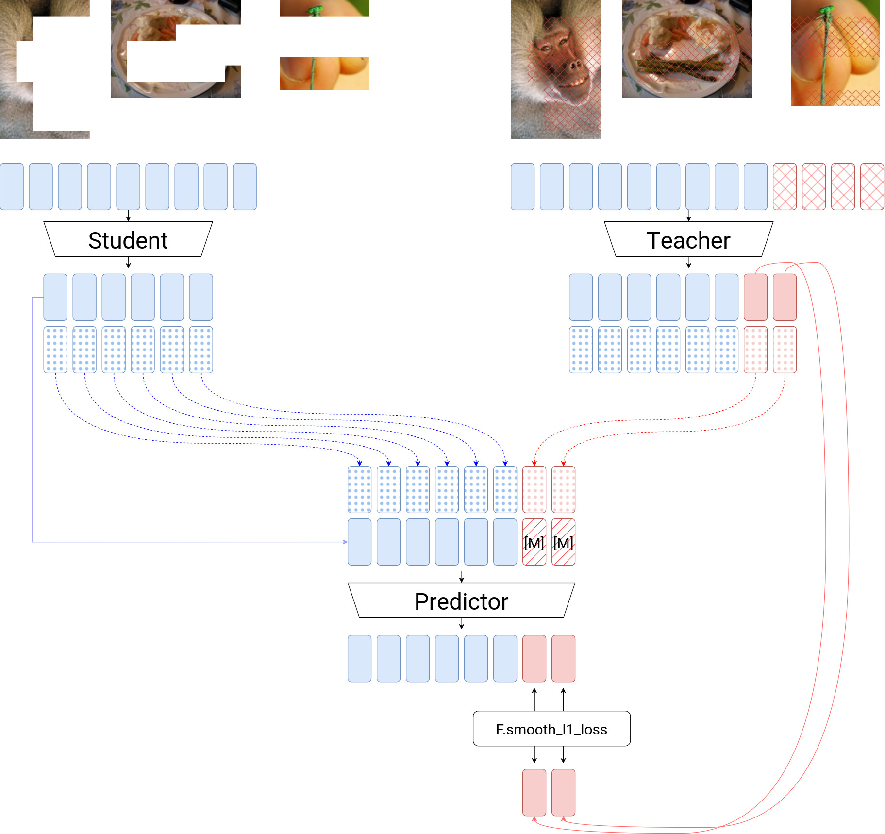
The student processes the tokens that are part of the context to produce context embeddings (solid blue) and position embeddings (dotted blue). The teacher processes the full set of tokens to produce embeddings and position embeddings. The predictor takes the position embeddings and embeddings from the context. The predictor also takes the position embeddings from the prediction targets (dotted red and solid red). The predictor uses a mask token ([M]) to indicate which tokens are prediction targets. The predictor estimates what the prediction targets are. Smooth l1 loss measures the distance between the predictions and the ground truth tokens outputted by the teacher. Notice that the number of tokens that the teacher and student output is not necessarily the same as the number of input tokens. This diagram represents the `wo unmerge` configuration.

Results

I train a ViT-S with a predictor of width 256 and depth 4. I follow the hyperparameters used in the original IJEPA paper. I use AdamW with a learning rate of 1e-3 and weight decay fixed at 0.05. The teacher's EMA beta starts at 0.996 and linearly increases to 1.0. All schedulers (including the EMA beta) are run as if the number of total training steps was extended by 1.25. I use 5,000 warmup steps, where the learning rate is increased from 2e-4 to 1e-3.

The original IJEPA code has a lower number of images per training step than the IJEPA-enhanced training runs. I do not change the original IJEPA code at all apart from adding a ViT-S configuration. IJEPA finished 60 epochs in 300k steps.

All IJEPA-enhanced runs had the same number of average images per training step, at about 520, completing 20 epochs in 50k training steps. The 50k training run and single evaluation run take about 6.5 hours.

Discussion

wo unmerge results in a remarkably higher throughput. It also has much lower memory usage. Too bad it gets only 17% linear probing accuracy. I want to find a fix that allows it to get comparable accuracy.

w unmerge and no merging whatsoever has nearly identical training throughput. When training larger ViTs or when training at higher resolutions, w unmerge becomes faster than no merging. There's a small reduction in linear probing accuracy but this could be justified by the increased efficiency.

I'd say that IJEPA-enhanced is a contender for the best low resource method for quickly training a self supervised ViT. But there are still some unexplainable observations that I have. For one, the linear probing accuracy starts to decrease after about 50,000 steps. I don't think this is a result of overfitting; the linear probing accuracy on the TRAINING set also decreases. Additionally, I did a short test training on DFN-200m, a larger image dataset. I also saw the same decrease in linear probing accuracy, despite not even completing one training epoch. This decrease also occurred in my training run I did with the official IJEPA code.

Thanks for reading this report. I want to further refine the techniques I used in IJEPA-enhanced. There's huge potential in the IJEPA-style masked latent prediction. If you want to collaborate with me, send me a message at atcolton@tutanota.com