A Theory for Coupling Generation and Compression

The Current Generation Paradigm: Decomposer and Generator

The design of almost every generative model follows the same pattern. First a decomposing model is trained (or hand coded) to compress instances of the particular data source. Only after ensuring that the compressed data can be accurately and predictably decompressed is the generative model trained to generate instances of the compressed data.

This paradigm holds for LLMs. Tokenizers compress a byte stream into a lower number of tokens. The information content of tokenized text is lower than raw text. It can lead to issues with the LLM not being able to understand how sub character spelling works. But tokenization is still worth it because it sufficiently speeds up the training and inference.

This paradigm is extremely common for image generators. Various types of decomposing models exist, from VQGANs to VAEs to JPEG bits. Similar to tokenizers for LLMs, the decomposer compresses the pixel data in order to save the generator from dealing with the nitty gritty of unneccesary low level granular details.

Using a hierarchy of models complicates things. It is worth it because it saves money. Even though the mapping learned by the decomposer is almost always lossy, this is acceptible because the decomposer speeds up the generator by so much.

Problem formulation

Let $x \in \mathbb{R}^d$ be a random variable distributed according to a target distribution $p^*$. Let's say that $p^*$ is images of dogs. I'll call the training set $D=\set{x_1, ..., x_n}$, which consists of i.i.d. images of dogs.

The decomposer is a parameterized function $d_\pi(\cdot;\theta):\mathbb R ^d -> \mathbb R ^k$. It maps high dimensional data into lower dimensional data. I differ from a typical formulation by allowing the decomposer to be conditioned on the generators parameters, $\pi$. The decomposer is used to make a latent dataset $Z=\set{d_\pi (x_1;\theta ), ..., d_\pi (x_n;\theta )}$.

The generator is another parameterized function. From a bayesian perspective the generator models the conditional distribution $p_\theta(x|z)$. The generator uses the latent space to model the probability distribution of the original input space $p_\theta(x)=\int p_\theta (x|z)p(z)dz$

The generator and decomposer are trained seperately. First the decomposer is trained, and then the generator. Remember that training both models together is only impossible because it's too expensive. If you had the budget to train the decomposer and generator together, you'd in effect be training one big generator. Instead the idea is to train as big a decomposer as compute permits, then compress the dataset to latents with a one-time cost, then train as big a generator as possible on the latents.

If you squint your eyes a little bit, this setup is a bilevel optimization problem. The decomposer (leader) optimizes π while anticipating the generator's response. The ideal decomposer takes into account how effectively the generator uses $Z$ to model the input data. The generator (follower) optimizes θ given the latent representations.

Approximating Predictability

Bilevel optimization isn't popular because it is expensive and complicated. But looking at image generation through the perspective of bilevel optimization can give us some insights as to how we can allow the decomposer and generator to work together more efficiently.

For instance, the most famous decomposer is the variational auto encoder (VAE). VAEs use a KL-regularization to make the latent variable z more predictable. This makes a lot of since since the whole point of the decomposer is to produce simple and predictable latents for the generator. But if we know the architecture that the downstream generator will use, we can discard KL-regularization for a more faceted estimate of predictability.

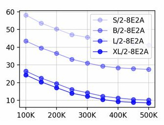FID vs number of training steps for different model scales, taken from Scaling Diffusion Transformers to 16 Billion Parameters The generator's quality increases very predictably as a function of model size and training steps.

My idea is for the decomposer to ditch old regularization in favor of a new regularization which directly optimizes an estimation of the downstream quality of the latents. The decomposer gets jointly trained with a small generator. The generator is a tiny version of the big generator that gets trained later. The tiny generator's loss value can be extrapolated to predict the big generator's loss. If the tiny generator generates $\hat z_{tiny}$, you can estimate what the big generator would generate, $\hat z$. Now you can directly use $\hat z$ for the decomposer. The whole setup looks like this.

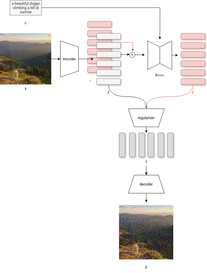Encode x to latent tokens using the encoder. Noise the tokens and use the tiny generator to try and predict the noise conditioned on the text prompt. The regularizer uses the distortion added by the tiny generator to predicts the distortion that the big generator will have. The decoder is given latents that are distorted in the same way that the big generator will distort them, and needs to decode them back to something close to the original pixels.